How to Make a Heat Map in Excel: Step by Step
To make a heat map in Excel, select the range of numbers you want to color. On the Home tab, select Conditional Formatting > Color Scales, and pick a color scale. Excel shades each cell by its value, so high and low numbers stand out at a glance.
This guide covers how to set up your data, apply a two-color or three-color scale, and customize the rule. It also shows how to hide the numbers for a cleaner look. It also covers heat maps from PivotTables, map charts for states and postal codes, and a worked example. Steps come from Microsoft's support pages, read on November 17, 2026.
What a heat map in Excel is
A heat map is a grid of numbers where color shows the size of each value. Dark or warm colors mark high values, and light or cool colors mark low ones. Your eye finds the hot spots before you read a single number.
Excel does not have a chart type with that name. Instead, you build one with conditional formatting. Microsoft explains that "Color scales are visual guides that help you understand data distribution and variation."
The format works well for data with two dimensions, such as:
- Sales by region and month. Spot the strongest markets and the slow months.
- Website visits by weekday and hour. Find the busiest times.
- Survey scores by question and team. See where satisfaction is low.
- Test results by student and topic. Find the topics that need more teaching.
- Risk ratings by likelihood and impact. Build a simple risk matrix.
If your data is a single list, a heat map still works, but a bar chart may be clearer. The format shines when you scan rows and columns together.
Set up your data
A heat map needs a clean grid. Put one category down the rows and another across the columns. Fill the inside with numbers.
| Jan | Feb | Mar | |
|---|---|---|---|
| North | value | value | value |
| South | value | value | value |
| East | value | value | value |
Follow three rules:
- Numbers only inside the grid. Text or error values break the color logic.
- Same unit everywhere. Do not mix dollars and percentages in one heat map.
- No totals inside the colored range. A total row is much larger than the other cells and will swamp the colors. Keep totals outside the selection.
If a cell holds a formula that might return an error, fix it first. Microsoft notes that if any cells in the selection "contain a formula that returns an error, the conditional formatting is not applied to those cells." It suggests using an IS or IFERROR function so the formula returns a value instead.
Apply a color scale
This is the core step. It takes less than a minute.
- Select the numbers in your grid. Do not include the row or column labels.
- On the Home tab, in the Styles group, select Conditional Formatting.
- Select Color Scales.
- Hover over the options to preview them, then click the one you want.
Microsoft's quick formatting steps match these. It says to "click the arrow next to Conditional Formatting, and then click Color Scales."
Excel offers two kinds of color scale:
- Two-color scale. Microsoft says it "helps you compare a range of cells by using a gradation of two colors." Use it when you only care about high versus low.
- Three-color scale. It uses "a gradation of three colors" to show "higher, middle, or lower values." Use it when the middle matters, such as targets or averages.
A common choice is green-yellow-red, with green for good values. For data where high is bad, such as costs or error rates, reverse it so red marks the high values.
Customize the color scale rule
The preset scales use the lowest and highest values in your range. You can change that, along with the colors.
- Select the grid, then select Conditional Formatting > Manage Rules.
- Select the color scale rule, then select Edit Rule.
- In Format Style, pick 2-Color Scale or 3-Color Scale.
- For Minimum, Midpoint, and Maximum, choose a Type and a Color.
Microsoft lists several types for these points:
- Lowest Value and Highest Value use the actual range of your data.
- Number lets you set fixed values, such as a target of 100.
- Percent spreads colors in proportion, with valid values "from 0 (zero) to 100."
- Percentile helps when a few extreme values would distort the colors.
- Formula lets you calculate the points, such as the average of the range.
Percentile is the most useful fix for skewed data. Microsoft says to use it when you want to show the top group "in one color grade proportion" and the bottom group in another. Extremes can "skew the visualization of your data," and percentiles stop that.
Microsoft also warns: "Make sure that the Minimum value is less than the Maximum value."
Choose colors that everyone can read
Color does all the work in this kind of chart, so the palette matters. A few choices make the grid easier to read for everyone.
Avoid red and green alone. Many people with color vision deficiency struggle to tell red from green. A blue-to-orange scale, or a single color from light to dark, is safer. If you keep green and red, show the numbers too.
Use one color for one direction. A white-to-dark-blue scale is often clearer than three colors. Darker simply means more. Keep three-color scales for data with a meaningful middle, such as a target or zero.
Keep the background light. Very dark cells make black numbers hard to read. Switch the font to white for the darkest cells, or lighten the top color.
Print a test copy. Colors that look fine on screen can merge on a gray printer. If the grid will be printed, check it in grayscale first.
Match your brand or report style. Pick colors that fit the rest of the document. Under More Colors in the rule editor, you can enter exact color codes.
Hide the numbers for a cleaner heat map
Sometimes you want only colors, like a true visual heat map. You can hide the numbers without deleting them.
- Select the colored grid.
- Press Ctrl+1 to open Format Cells.
- On the Number tab, select Custom.
- In the Type box, enter three semicolons:
;;; - Select OK.
The values stay in the cells, so the colors and any formulas still work. They just do not show. Click a cell to see its value in the formula bar.
To make the grid look like a block of tiles, narrow the columns and set the row height to match. Remove gridlines under View > Gridlines for a cleaner finish.
Keep a legend or a note explaining the colors. A heat map without a legend leaves readers guessing what dark green means.
Make a heat map from a PivotTable
Most real data does not arrive as a neat grid. It comes as a long list, with one row per sale or visit. A PivotTable turns that list into a grid you can color.
- Select your data, then select Insert > PivotTable.
- Drag one field, such as Region, to Rows.
- Drag another field, such as Month, to Columns.
- Drag the number field, such as Sales, to Values.
- Select the value cells and apply a color scale.
Microsoft notes that you can apply color scales to "a range, table, or PivotTable report." When you apply one to a PivotTable, a Formatting Options button appears. Use it to apply the rule to all cells for that value, excluding subtotals and grand totals.
This is the best way to build a heat map with two variables from raw data. When the source data changes, refresh the PivotTable and the colors update.
For a refresher, see our guide on how to make a pivot table in Excel.
Make a geographic heat map with a map chart
If your rows are places, such as states or postal codes, you may want colors on a real map. Excel's map chart does this.
Microsoft says to use a map chart "when you have geographical regions in your data, like countries/regions, states, counties or postal codes." It adds that this feature is available "if you have a Microsoft 365 subscription."
- Put the place names in one column and the values in the next.
- Select any cell in the data.
- Go to Insert > Charts > Maps > Filled Map.
For values, Microsoft says the map uses "slight variations of two to three colors." By default, "the higher the value is, the darker its corresponding color will be."
Map charts work best for regions Excel recognizes, such as countries and states. Street addresses need extra steps, so a grid heat map is often simpler for city-level data.
A worked example: sales by store and month
Here is a grid built from monthly sales, in thousands of dollars, for four stores.
| Store | Jan | Feb | Mar | Apr | May | Jun |
|---|---|---|---|---|---|---|
| North | 52 | 48 | 55 | 61 | 66 | 70 |
| South | 38 | 35 | 40 | 44 | 43 | 47 |
| East | 61 | 64 | 59 | 72 | 78 | 81 |
| West | 29 | 31 | 30 | 33 | 35 | 34 |
Select B2:G5 and apply a green-yellow-red color scale, with green for high values. The pattern jumps out:
- East is the strongest store. Its June figure of 81 is the darkest green cell.
- West is the weakest. Its January figure of 29 is the deepest red.
- Every store grew from January to June, so the right side of the grid is greener.
- February dipped for North and South, which shows as a lighter band.
Without color, you would need to read all 24 numbers to see this. With color, it takes a few seconds. That speed is the whole point of the format, especially in a meeting where people glance at a slide for only a moment.
To focus on growth instead of size, add a second grid with each month's change. A three-color scale with the midpoint at zero then shows growth in green and decline in red.
Make a heat map in Excel with AI
The steps above are quick once the grid exists. Building the grid from raw exports, picking the right fields, and spotting the story takes longer. An AI tool can do that work for you.
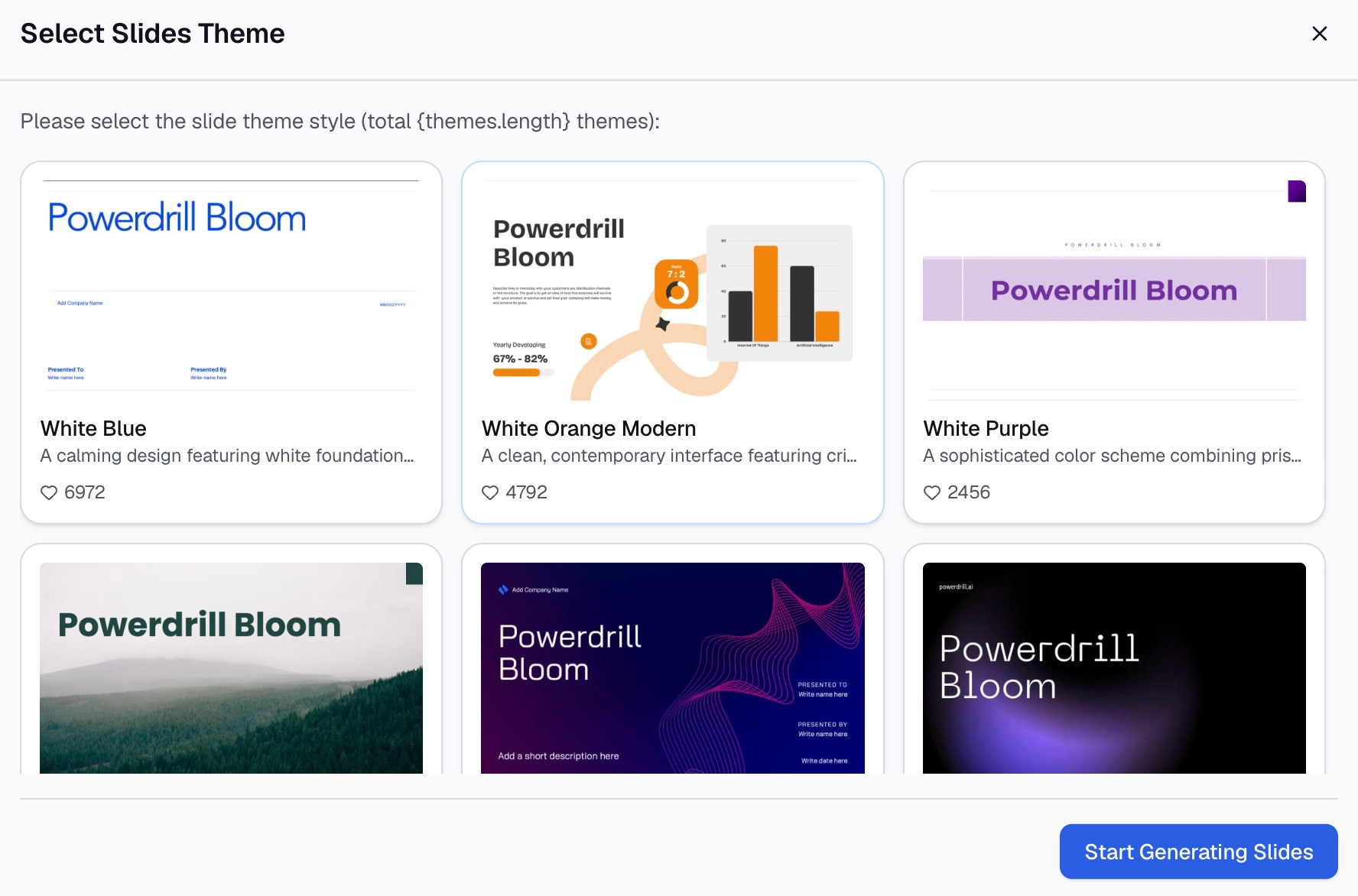
Here is the method in three steps, using Powerdrill Bloom.
Step 1: Upload your Excel or CSV file
Upload the file with your raw data, such as a sales export with one row per order. The Make Graphs from Excel page says the tool "supports multiple file formats: Excel, CSV, or PDF."
You do not need to build a PivotTable first. The tool can group the rows for you.

Step 2: Ask for the heat map in natural language
Describe the grid you want. For example: "Make a heat map of sales by store and month, with darker colors for higher sales."
Our data visualization tool can turn data into visuals "such as Bar, Line, Pie, Doughnut, Heatmap, Boxplot, and more." Ask it to point out the highest and lowest cells, too.
Step 3: Review the chart and share it
Check a few cells against your source data. Then keep the chart for your report or slides.
The Make Graphs from Excel page says you can turn the results "into PPT slides, infographics, or Notion pages." Rebuild the color scale in Excel if you need the heat map in a workbook.
Common mistakes to avoid
These are the problems that come up most often with a heat map in Excel.
- Including totals. A total row dominates the colors. Exclude it from the selection.
- Mixing units. One heat map should use one unit only.
- Wrong color direction. For costs or errors, high values should look bad, not good.
- Extreme values. One huge number washes out the rest. Use percentiles for the scale points.
- Too many colors. Two or three colors are easier to read than a rainbow.
- No legend. Tell readers what the colors mean.
- Formula errors. Cells with errors stay uncolored. Wrap formulas in IFERROR.
For a version built from raw spreadsheet data, see our guide on how to make a heatmap from spreadsheet data with AI. For another chart that shows spread, see how to make a box plot in Excel.
When your data sits in a long export, try Powerdrill Bloom and ask for the heat map in one sentence.
Frequently asked questions
Does Excel have a heat map chart?
Excel has no chart named heat map. You create one with conditional formatting color scales on a grid of numbers. For geographic data, a Filled Map chart works like a heat map.
How do I make a heat map in Excel with two variables?
Put one variable in the rows and the other in the columns, with values in the grid. A PivotTable builds this grid from raw data. Then apply a color scale.
How do I change the colors in an Excel heat map?
Select the grid, then select Conditional Formatting > Manage Rules > Edit Rule. Choose new colors for the minimum, midpoint, and maximum.
Can I make a heat map without showing the numbers?
Yes. Apply a custom number format of three semicolons (;;;). The values stay in the cells, but only the colors show.
Can I make a heat map in Excel with states or zip codes?
Yes. Use Insert > Charts > Maps > Filled Map with a Microsoft 365 subscription. Excel colors each state or postal code by its value.
Sources: Microsoft Support, Use conditional formatting to highlight information in Excel · Microsoft Support, Create a Map chart in Excel.