How to Make a Dashboard in Google Sheets: Step by Step
To make a dashboard in Google Sheets, keep your raw data on one tab. Build summary tables on a second tab with SUMIF or a pivot table. On a third tab, add charts with Insert > Chart, including scorecard charts for key numbers. Then add a slicer with Data > Add a slicer, so viewers can filter every chart at once.
This guide walks through each step, from structuring the data to sharing the finished dashboard. It also covers scorecard charts, slicers, automatic updates, and a worked sales example. Steps come from the Google Docs Editors Help Center, read on November 17, 2026.
What a Google Sheets dashboard is
A dashboard is a single screen that shows the numbers a team checks most often. Instead of scrolling through rows, readers see totals, trends, and comparisons in a few charts.
Google Sheets is a good home for a simple dashboard when:
- Your data already lives in Sheets. Sales logs, form responses, budgets, or exports.
- Several people need to see it. Sharing a link is easier than emailing files.
- You want it to stay current. Charts update when the data changes.
- You do not have a BI tool. Sheets is free and familiar.
A good dashboard answers three to five questions at most. For example: How much did we sell? Is it up or down? Which region leads? Which product lags? Decide your questions before you build anything.
For heavier needs, such as millions of rows or data from many systems, a dedicated BI tool is a better fit. For most team reports, a Sheets dashboard is plenty.
Plan the layout with three tabs
The most reliable dashboards in Google Sheets use three tabs. Each has one job.
| Tab | What goes on it | Who edits it |
|---|---|---|
| Data | Raw rows, one record per row | Imports, forms, or data entry |
| Calc | Summary tables and formulas | You, once during setup |
| Dashboard | Charts, scorecards, and slicers | Nobody, after setup |
This split keeps things stable. New data goes only into the Data tab. Formulas on the Calc tab pick it up. Charts on the Dashboard tab read from Calc, so they update without anyone touching them.
Sketch the dashboard on paper first, or in a blank slide. A rough drawing saves rework later. Put the most important numbers across the top as scorecards. Put trend charts in the middle and detail charts below. Leave space at the top for slicers.
Prepare the data tab
Charts are only as clean as the data behind them. Set up the Data tab carefully.
- One header row. Give each column a short, clear name, such as Date, Region, Product, Units, and Revenue.
- One record per row. Each sale, response, or transaction gets its own row.
- No blank rows or merged cells. They break formulas and pivot tables.
- Consistent values. Use the same spelling for each region and product.
- Real dates and numbers. Format dates as dates and amounts as numbers, not text.
Google's pivot table guide stresses one of these rules: "Each column needs a header."
Freeze the header row with View > Freeze > 1 row. That keeps column names visible as the data grows.
If your data comes from a form or another system, import it here and leave it untouched. Do your cleaning and math on the Calc tab.
Build summary tables on the Calc tab
Charts work best when they read from small summary tables, not thousands of raw rows. Build those tables on the Calc tab with formulas or a pivot table.
Option 1: SUMIF formulas. Google describes SUMIF as a function that "Returns a conditional sum across a range." The syntax is SUMIF(range, criterion, [sum_range]).
List your regions in column A of the Calc tab. In B2, total revenue for the first region:
=SUMIF(Data!B:B,A2,Data!E:E)
Copy it down for each region. Here Data!B:B holds the region and Data!E:E holds revenue.
Option 2: A pivot table. Pivot tables build summaries without formulas.
- Select your data on the Data tab.
- Select Insert > Pivot table, and place it on the Calc tab.
- In the side panel, add Region under Rows.
- Add Revenue under Values, summarized by SUM.
Google notes that Sheets may suggest pivot tables, and that "High confidence pivot table suggestions will be automatically inserted upon pivot table creation." Check any suggestion before you rely on it.
Option 3: QUERY. For more control, the QUERY function "Runs a Google Visualization API Query Language query across data." For example, =QUERY(Data!A:E,"select B, sum(E) group by B") totals revenue by region in one formula.
Add charts to the dashboard tab
With summary tables ready, the charts come together quickly. Google's steps are short:
- Select the cells you want to include in your chart.
- Click Insert > Chart.
- In the chart editor, under Chart type, choose the type you want.
Move each chart to the Dashboard tab. Click the chart, open the three-dot menu, and select Move to own sheet, or cut and paste it.
Pick chart types by question:
| Question | Chart type |
|---|---|
| How did it change over time? | Line chart |
| Which group is biggest? | Bar or column chart |
| What share does each part hold? | Pie or donut chart, with five slices or fewer |
| What is the single key number? | Scorecard chart |
| How do two measures relate? | Scatter chart |
Give each chart a title that states the finding, such as "East leads revenue this quarter." Remove gridlines and legends you do not need. Use one consistent color for each category across every chart on the dashboard.
Show key numbers with scorecard charts
Scorecards are the headline numbers at the top of a dashboard. Google says they "Call attention to key performance indicators, known as KPIs," like "total sales, average cost, or a top selling item."
To add one:
- Click Insert > Chart.
- In the chart editor, under Chart type, scroll to Other and choose Scorecard chart.
- On the Setup tab, under Key value, select the cell or range.
If you select a range, Google says you can display information "like sum or average." Choose the option under Aggregate.
Scorecards can also compare two numbers. Google explains that you can "compare two ranges of data to show differences, like changes over time." Under Baseline value, select last period's total. The scorecard then shows the change next to the key value. To show the change as a percentage, use the Customize tab.
Three or four scorecards across the top is a good number. More than that and the eye does not know where to start.
Pick scorecards that a reader can act on. Total revenue, orders, and average order value work well for a sales team. Open tickets, average response time, and satisfaction score suit a support team. For a budget, use spending to date, the remaining budget, and the largest overspend. Each one should map to a question from your plan.
Format scorecard numbers so they read at a glance. Round large values, such as 425K instead of 425,000. Under the Customize tab you can change the font size, color, and number format.
Add slicers to filter the dashboard
A slicer turns a static report into an interactive one. Google says that on a custom dashboard, "you can add a slicer to filter your tables, charts, or pivot tables."
- Click a chart or pivot table on the dashboard.
- At the top, click Data > Add a slicer.
- On the right, choose a column to filter by, such as Region.
- Click the slicer and choose your filter values.
One slicer can control many charts. Google notes that slicers "apply to all charts and pivot tables in a sheet that use the same data set."
Keep two limits in mind. Google says slicers "don't apply to formulas in a sheet that use the same data set." SUMIF tables will not respond, so point charts at pivot tables if you want them filtered. Also, "You can use one slicer per column," so add one slicer for each field you want to filter.
A slicer's choices are private to each viewer unless you set them as the default. That lets several people explore the same dashboard without changing what others see.
A worked example: a quarterly sales dashboard
Here is a simple dashboard for a sales team's third quarter. The Data tab holds 1,200 order rows with Date, Region, Product, Units, and Revenue.
The Calc tab sums revenue by region with SUMIF:
| Region | Revenue (USD) |
|---|---|
| North | 120,000 |
| South | 95,000 |
| East | 140,000 |
| West | 70,000 |
| Total | 425,000 |
The Dashboard tab then shows:
- Scorecard: total revenue. Key value 425,000, with last quarter's 400,000 as the baseline. It shows growth of 6.25%.
- Scorecard: units sold. A sum of the Units column.
- Column chart: revenue by region. East is the tallest bar and West the shortest.
- Line chart: weekly revenue. It shows a dip in week 6 and a strong finish.
- Slicer: Region. Viewers can pick one region to see its trend.
The story fits on one screen, and nobody has to open the Data tab to follow it. Revenue grew 6.25% over last quarter. East leads with about a third of the total, and West trails at about one sixth. That points the next sales meeting at West's pipeline.
Keep the dashboard updated and share it
A dashboard is useful only if people trust that it is current.
- Feed the Data tab automatically. Link a Google Form, or use IMPORTRANGE to pull from another sheet.
- Use open-ended ranges. Formulas such as
Data!E:Einclude new rows without edits. - Refresh pivot ranges. If a pivot table uses a fixed range, extend it as data grows.
- Protect the Calc and Dashboard tabs. Right-click a tab and choose Protect sheet so nobody breaks a formula.
- Add a last-updated note. A cell such as "Data through November 16, 2026" sets expectations.
To share, click Share and give view access. For a wider audience, you can publish. Google says that after you publish, "you can send a new URL to anyone or embed into your website." It also warns that published charts "show the data used to create them," so check for private information first.
For a newer layout option, see our guide to Google Sheets canvas.
Make a dashboard in Google Sheets with AI
Building the tabs takes an hour or two the first time. Choosing which numbers matter, and keeping the charts current across messy exports, takes longer. An AI tool can do the analysis and draft the charts for you.
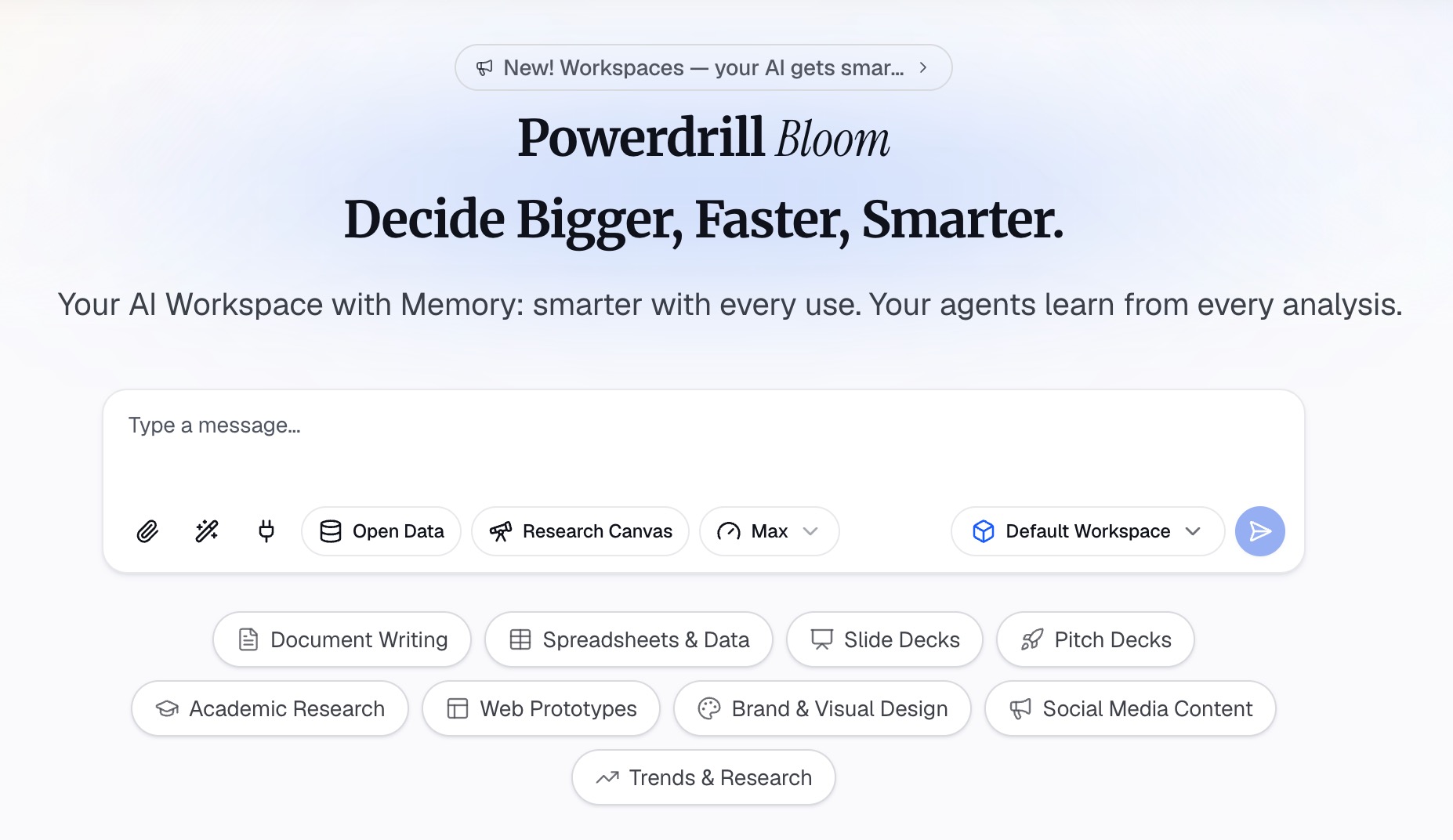
Here is the method in three steps, using Powerdrill Bloom.
Step 1: Upload your exported sheet
Download your Google Sheet as an Excel or CSV file, and upload it. Our data visualization tool lets you drop in your files and ask "anything you want from your data."
Upload the raw Data tab. You do not need to build the Calc tab first.
Step 2: Ask for the dashboard in natural language
Describe the dashboard you want. For example: "Build a dashboard with total revenue, revenue by region, and weekly revenue trend for Q3."
The tool page says you can "Customize and save these charts to suit your needs, then add them to dashboards." Ask it to point out the biggest changes, too.
Step 3: Review the charts and rebuild the best ones in Sheets
Check each number against your Calc tab. Keep the charts and findings that answer your questions.
Then rebuild those charts in your Google Sheets dashboard, so they update with live data. For a related walkthrough, see our guide on how to build a KPI dashboard from a spreadsheet.
Common mistakes to avoid
These are the problems that come up most often with a dashboard in Google Sheets.
- Too many charts. Limit the screen to the questions that matter.
- Charts on raw data. Point charts at summary tables, not thousands of rows.
- Mixed spellings. Inconsistent values split one region into two.
- Slicers on formulas. Slicers do not filter SUMIF tables. Use pivot tables for filtered charts.
- No baseline. A number without a comparison does not tell readers if it is good.
- Unprotected tabs. One stray edit can break every chart.
- Publishing sensitive data. Published charts show their data. Check before you publish.
For more on charts in Sheets, see our guide on how to turn Google Sheets data into charts with AI.
When your data sits in a long export, try Powerdrill Bloom and ask for a first draft of the dashboard.
Frequently asked questions
Does Google Sheets have a dashboard feature?
Google Sheets has no single dashboard button. You build one from charts, scorecard charts, pivot tables, and slicers, usually on a dedicated tab.
How do I make an interactive dashboard in Google Sheets?
Add slicers with Data > Add a slicer. Slicers filter every chart and pivot table that uses the same data set, so viewers can explore by region, product, or date.
How do I make a Google Sheets dashboard update automatically?
Keep raw data on one tab and use formulas or pivot tables that read open-ended ranges. Feed the data tab from a Google Form or IMPORTRANGE.
What is a scorecard chart in Google Sheets?
A scorecard chart shows one key number, such as total sales, in large type. It can also compare that number with a baseline, such as last month.
Can I share a Google Sheets dashboard with people outside my team?
Yes. Share the file with view access, or publish it to get a link or embed code. Published charts show their data, so check for private information first.
Sources: Google Docs Editors Help, Add & edit a chart or graph · Google Docs Editors Help, Display KPIs with scorecard charts · Google Docs Editors Help, Filter charts and tables with Slicers · Google Docs Editors Help, Create & use pivot tables · Google Docs Editors Help, SUMIF · Google Docs Editors Help, QUERY function · Google Docs Editors Help, Make Google Docs, Sheets, Slides & Forms public.