How to Make a Pivot Chart in Excel: 3 Easy Ways in 2026
To make a pivot chart in Excel, select a cell in your data, go to Insert, and choose PivotChart. Pick where the chart should go, select OK, and then choose the fields to show. Excel builds a PivotTable and a linked chart at the same time.
This guide covers three ways to make a pivot chart: straight from your data, from an existing PivotTable, and in Excel for the web. It also covers how to filter, change, and fix a pivot chart, plus a faster way to chart large files. Steps come from Microsoft's support pages, read on November 12, 2026.
What a pivot chart is
A pivot chart is a chart built on top of a PivotTable. Microsoft says "PivotCharts provide graphical representations of the data in their associated PivotTables."
The two stay linked. Microsoft's overview says changes to an associated PivotTable "are immediately reflected in the layout and data in the PivotChart and vice versa."
That link is what makes the chart useful. You can drag a field into the chart, and the summary and the picture update together. A normal chart points at fixed cells and does not regroup data for you.
Microsoft's own reason for using one is simple. It says "not everyone can look at numbers in a table and quickly see what's going on."
A pivot chart is a good fit when:
- You have many rows to summarize. Hundreds of sales lines become a few bars by region.
- You want to compare groups. Units by product, costs by department, or tickets by team.
- The questions keep changing. A manager asks by region today and by product tomorrow.
- The data grows each month. New rows flow in when you refresh an Excel table.
It is a poor fit for a single fixed chart that never changes. A regular chart is simpler to format in that case.
Pivot chart vs. regular chart
Most chart tools work the same way in both. Microsoft lists a few differences worth knowing before you start.
| Feature | Pivot chart | Regular chart |
|---|---|---|
| Data source | The associated PivotTable | Worksheet cells |
| Change the data range | Not from Select Data Source | Yes, from Select Data Source |
| Switch rows and columns | Pivot the PivotTable fields instead | Yes, from Select Data Source |
| Chart types | Any type except xy (scatter), stock, or bubble | Any type |
| Filtering | Built-in PivotChart Filter Pane | Manual filters on the source data |
| Formatting on refresh | Trendlines, data labels, and error bars are not kept | Formatting stays |
The last row catches many people. Microsoft says that on refresh, "trendlines, data labels, error bars, and other changes to data sets are not preserved." Add those finishing touches last, or reapply them after a refresh.
Set up your data first
A pivot chart is only as good as the data under it. Microsoft gives clear rules for source data.
- Use list format. Put "column labels in the first row," which Excel uses for field names.
- One type per column. Microsoft says "you shouldn't mix data types in the same column."
- No gaps. There "shouldn't be any blank rows or columns within the data range."
- Use an Excel table. Microsoft notes that new data in a table is included when you refresh the PivotTable.
Here is a small sales table used in the examples below:
| Month | Region | Product | Units |
|---|---|---|---|
| Jan | North | Desk | 120 |
| Jan | South | Desk | 90 |
| Jan | North | Chair | 200 |
| Feb | South | Chair | 160 |
| Feb | North | Desk | 140 |
| Feb | South | Desk | 110 |
To turn it into a table, select any cell and press Ctrl+T. Name the table something short, such as Sales, so you can find it later. If your data starts as an export from another system, scan it before you build anything. Delete subtotal rows, unmerge merged cells, and make sure every month is written the same way. Ten minutes of cleanup here saves a confusing chart later.
Way 1: Create a pivot chart straight from your data
This is the fastest way on Windows. Excel creates the PivotTable and the chart together.
Follow Microsoft's steps:
- Select a cell in your table.
- Select Insert and choose PivotChart.
- Select where you want the PivotChart to appear.
- Select OK.
- Select the fields to display in the menu.
For the sales table, drag Region to the Axis area and Units to the Values area. Excel sums the units by region and draws a column chart.
Next, drag Product to the Legend area. The chart now splits each region's bar by product. You have built a grouped comparison without writing one formula.
Excel places the PivotTable and chart on the sheet you chose in step 3. Most people pick a new worksheet so the summary does not crowd the raw data.
Way 2: Create a pivot chart from an existing PivotTable
If you already have a PivotTable, you can chart it directly. This is also the only route on a Mac.
On Windows, the steps are short:
- Select a cell in your PivotTable.
- Select Insert and choose PivotChart.
- Select a chart.
- Select OK.
On a Mac, Microsoft says "you need to create a PivotTable first, and then insert a chart." Select any cell in the PivotTable, then use the Insert tab.
The Mac has a limit on chart types. Microsoft says you can insert "either a column, line, pie, or radar chart." It adds that "other types of charts do not work with PivotTables at this time," such as treemap, statistical, and combo charts.
Once the chart is in place, it behaves like a PivotChart. Microsoft says it will update "if you change the fields in the PivotTable Fields list."
If you need a refresher on the table itself, our guide on how to make a pivot table in Excel walks through each field area.
Way 3: Create a pivot chart in Excel for the web
Excel for the web also needs a PivotTable first. Microsoft says "you will first need to create a PivotTable."
Then follow these steps:
- Select a cell in your PivotTable.
- On the Insert tab, open the Insert Chart dropdown menu.
- Select any chart option.
The chart appears on the worksheet. When you select it, a Chart tab appears in the ribbon with options to change the design.
This route works well for shared workbooks in OneDrive or SharePoint. Several people can view the same chart without installing desktop Excel.
Excel for the web has fewer options than the desktop app. If a menu you need is missing, open the file in desktop Excel from the Editing menu, make the change, and save it back.
Filter and change your pivot chart
The main reason to use a pivot chart is to explore. Microsoft says "When you create a PivotChart, the PivotChart Filter Pane appears." You can use it to sort and filter the data under the chart.
Here are the changes people make most often:
- Filter one value. Open the filter on Region and keep only North. The chart and table both update.
- Add a slicer. Microsoft notes you can use slicers on the PivotTable, and "the chart will also be filtered."
- Change the chart type. Select the chart, then choose Change Chart Type. Any type works except xy (scatter), stock, or bubble.
- Swap the axis. Move Product to the Axis area and Region to the Legend area to flip the comparison.
- Group dates. Right-click a date field in the PivotTable and group by month or quarter.
To refresh after the source data changes, right-click the PivotTable and choose Refresh. The chart updates with it.
Format the chart for a report
A raw PivotChart works for exploring. A chart for a report or a slide needs a little more care. Microsoft says PivotCharts let you change "the titles, the legend placement, the data labels, the chart location, and so on."
Work through these finishing steps in order:
- Add a clear title. Replace the default Total label with a sentence such as "North sold 100 more units than South."
- Label the axes. Name the value axis with its unit, such as Units sold.
- Hide the field buttons. On the PivotChart Analyze tab, use the Field Buttons menu to hide them, so the chart looks clean on a slide.
- Pick a calm style. Use one color per series and remove heavy gridlines.
- Add data labels last. Labels are not kept after a refresh, so add them once the data is final.
To move the chart to its own sheet, right-click it and choose Move Chart. A chart sheet prints on one page and is easy to copy.
To use the chart in PowerPoint, copy it from Excel and paste it on a slide. Keep the source workbook saved, so you can refresh the numbers next month. Our guide on how to update PowerPoint charts from Excel covers the linking options.
Keep each chart focused on one question. If you need to answer three questions, make three small charts. One crowded chart with every field in it tends to hide the answer.
A pivot chart example
Here is how the sales table from earlier looks after Way 1. Region is on the axis, Product is in the legend, and Units is the value.
| Region | Chair | Desk | Total |
|---|---|---|---|
| North | 200 | 260 | 460 |
| South | 160 | 200 | 360 |
| Total | 360 | 460 | 820 |
The chart shows two clusters of bars. North sells 460 units in total, and South sells 360. In both regions, desks lead chairs.
Now add Month to the filter area and choose Feb. North shows 140 desk units and no chairs, while South shows 110 desks and 160 chairs. One filter changes the whole story.
That is the point of this kind of chart. Each new question takes a drag or a click, not a new chart.
Before you share the result, check that the totals match the source. Add a quick SUM under the Units column and compare it with the grand total in the PivotTable. If they differ, look for blank rows, text values, or rows outside the table range.
Make a pivot chart in Excel with AI
When a file has dozens of columns, choosing fields becomes the slow part. An AI tool can suggest the right grouping and draw the chart for you.
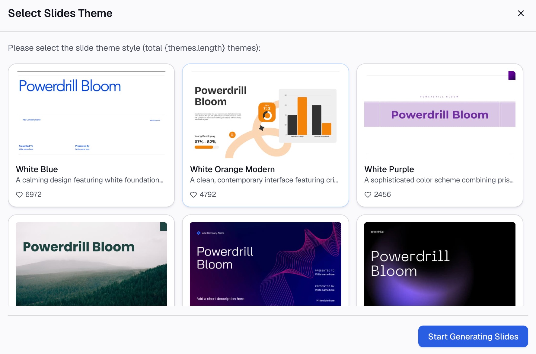
Here is the method in three steps, using Powerdrill Bloom.
Step 1: Upload your Excel file
Upload the workbook with your raw data. The Make Graphs from Excel page says to "Easily upload your Excel file containing the data you want to visualize." It supports Excel, CSV, or PDF files.
Keep the same tidy layout as above: one header row, one type per column, and no blank rows.

Step 2: Ask for the chart in natural language
Describe the summary you want. For example: "Show total units by region, split by product, as a column chart." Name the columns the way they appear in your file, so the AI picks the right fields.
The Vibe Data Analysis page says that "Whether it's a bar chart, line graph, or pivot table, Vibe creates dynamic visuals on the fly." You can then ask a follow-up, such as filtering to one month.
Step 3: Check the chart and export it
Check one total against the source data by hand. Then share the result. The Excel AI Assistant says you can "Export insights as PowerPoint slides, infographics, or Notion pages in one click."
For charts that go straight into a deck, the AI Graph Maker offers more chart styles.
Common mistakes to avoid
These are the problems that come up most often with PivotCharts.
- Blank rows in the source. Excel may stop the range early. Remove blank rows or use an Excel table.
- Numbers stored as text. They show as a count instead of a sum. Convert them to numbers first.
- Forgetting to refresh. The chart does not update when the source changes until you refresh.
- Losing labels on refresh. Data labels and trendlines are not kept, per Microsoft. Add them last.
- Too many categories. Twenty products in one legend is hard to read. Filter to the top few.
- Wrong chart type for the question. Use columns to compare groups and lines to show change over time.
- Expecting a scatter chart. PivotCharts cannot be xy (scatter), stock, or bubble charts.
- Mixing data types. A currency column with dates in it will break grouping.
For more ways to summarize data without building tables, see our guide on how to summarize Excel data without pivot tables.
When you are ready to chart a large file quickly, try Powerdrill Bloom with this month's sales export.
Frequently asked questions
How do I make a pivot chart in Excel?
Select a cell in your data, go to Insert, and choose PivotChart. Pick where the chart goes, select OK, and choose the fields to display. Excel creates the PivotTable and the pivot chart together.
Can I make a pivot chart without a PivotTable?
On Windows, Insert > PivotChart builds both at once, so you do not need to make the PivotTable first. On a Mac and in Excel for the web, you must create a PivotTable first.
Why can't I make a scatter pivot chart?
Microsoft says you can change a PivotChart to any chart type except xy (scatter), stock, or bubble. For a scatter chart, copy the PivotTable values and chart them as a normal range.
How do I refresh a pivot chart?
Right-click the PivotTable linked to the chart and choose Refresh. The chart updates at the same time, since the two are linked.
Why did my data labels disappear from my pivot chart?
Microsoft says trendlines, data labels, error bars, and other data set changes are not kept when you refresh a PivotChart. Reapply them after each refresh, or add them as the last step.
Sources: Microsoft Support, Create a PivotChart · Microsoft Support, Overview of PivotTables and PivotCharts.